CS 380 Lab 2: Species Distribution Modeling Using
MaxEnt (Part I)
The distribution of each species is determined by a combination of
factors, including climate, resources, and dependence on other
species. This unique combination of factors determines where
different species can live successfully. Even if a single species
could survive in a particular
climate and habitat, they may not have the resources to survive or
reproduce. Consider the following example by Park Williams (UCSB):
Consider Joshua trees, which are
confined to elevations between
400-1800 m (2,000-6000 ft.) in the Mojave Desert. To grow any lower
than 400 m or any further south than the Mojave Desert would be suicide
by drought. However, they grew lower in elevation and further south
during the cooler and wetter climate of the last glacial period. This
means that Joshua trees expand their range when they can. So why don’t
they live in coastal southern California? If a Joshua tree could take a
coastal vacation, it would likely find the climate to be ideal for
growth. However, it would never reproduce. To reproduce, Joshua trees
depend on a variety of yucca moth that is genetically programmed for
stuffing a little ball of pollen into the cup-shaped stigma of Joshua
tree flowers. This relationship is mutually vital for both plant and
moth, and for a complexity of reasons that are not fully understood,
the Mojave Desert is where these two species have been stuck with each
other since the beginning.
Our first guest speaker touched on the challenges of species
distribution modeling from both macro and micro perspectives. In
that presentation, we also saw some of the problems with MaxEnt for
prediction of species distributions. In this lab, you will
examine the effects of climate and climate change on the distributions
of several species of tree, and then use climate and species-range data
to construct computational models of species distribution using
MaxEnt. This lab will be split over two weeks, and will augment
our in-class discussions on MaxEnt and species distribution
modeling. You may (and should if at all possible) work with a
partner on this lab. You should submit only one copy of the lab
write-up for each group.
Examining Species Distributions
All files needed for this lab are available in ~eeaton/public/cs380/lab2/.
Examine the maps of California in ~eeaton/public/cs380/lab2/climate-maps.pdf,
each
of which depicts a single climate variables, such as mean annual
temperature, mean diurnal temperature range, mean precipitation during
the coldest quarter of the year, etc. Overlaid on each climate map are
maps of six species’ ranges: bigcone Douglas fir (Pseudotsuga
macrocarpa), Bishop pine (Pinus muricata), Blue oak (Quercus
douglasii), Jeffrey pine (Pinus jeffreyi), coast redwood (Sequoia
sempervirens), and giant sequoia (Sequoia giganteum).
Since later you will be placing graphics into your write-up, it would
be easiest to work in a format that supports this, such as LaTeX, MS
Word, or OpenOffice. Briefly
answer the following questions, typing up
your answers:
- Examine the first map (BIO1: Annual Average Temperature). Which
species appears to survive best in cold temperatures?
- The third map (BIO3: Isothermality) compares the day-to-night
temperature oscillation versus the
summer-to-winter temperature oscillation. A value of 100 would
represent a site
where the diurnal temperature range is equal to the annual temperature
range. A value of 50 would indicate a location where the diurnal
temperature range is half of the annual temperature range. Which region
has the highest isothermality (same temperate range)? What is a species
that appears to grow
well in a highly isothermal environment? What is a species that grows
across a range of isothermalities?
- Examine all of the 20 maps and choose two species to focus on for
the rest of the assignment. Note the two species you chose, and
examine the distribution of both species as they relate to the various
climate variables. Answer the remaining questions in this section
based on your two chosen species.
- Does your species appear to be confined to
regions with cool summers?
- Does a spatial pattern in annual rainfall
appear to correspond with the boundaries of any species’ range? Or is
rainfall only important during a specific time of year?
- For each of
your two species, what are the two climate variables that you
hypothesize to be most the most important in dictating that species’
distribution? Why have you chosen each climate variable?
Learning a Computational Model of Species Distributions using MaxEnt
MaxEnt was developed in a collaboration between machine learning
researchers and a biologist (emphasizing the interdisciplinary nature
of computational sustainability) in 2004. It is a recent
contribution from computer science / artificial intelligence that is
now used widely (as we saw in the first guest lecture) by biologists
and ecologists.
To learn the species distribution models, MaxEnt takes two inputs: (1)
a file containing exact locations where a species of interest is known
to grow and (2) a file containing climate data for each of those
locations. By evaluating the climate data at each location where
the species of interest is present, MaxEnt calculates a probability
function that describes the chances of a tree location having any given
climate setting. So if we were studying Joshua trees, MaxEnt would
predict that if a Joshua tree is growing in a given location, there is
a high probability that that location is hot rather than cold during
summer. Next, MaxEnt flips this probability function around to predict
the probability of species presence given a particular climate type.
Therefore, MaxEnt would predict a high likelihood of Joshua tree
presence in locations that are hot during summer and a low likelihood
of presence in locations that are cold during summer. While this
example focused on only one climate variable, MaxEnt generates the
model and predicts the presence likelihood using multiple climate
variables. We will examine precisely how MaxEnt learns the model
next week in class.
The data required by MaxEnt is included in the following three folders
under ~eeaton/public/cs380/lab2/:
environmentBaseTemp: the
20 climate parameters depicted in climate-maps.pdf
environmentIncrTemp: the 20 climate parameters, but with a
uniform increase of 4°C
speciesData: the species presence locations
The file ~eeaton/public/cs380/lab2/variables.pdf
contains textual descriptions of
each of the climate parameters.
To learn a computational model for the distribution of each of your two
species: (Read these directions completely before you build your
first model!)
- Run the MaxEnt program:
java -Xmx512M -jar ~eeaton/public/cs380/lab2/maxent/maxent.jar
- Input the file containing the presence locations for your first
species. Load this into the "Samples" section of the MaxEnt
program.
- Load the climate parameters into the "Environmental Layers"
section of the MaxEnt program by selecting the
environmentBaseTemp
folder.
- For this first species, you identified two climate parameters as
potentially important in determining the species' distribution.
Choose one of these climate parameters and select only the
environmental layer corresponding to that parameter. (Hint:
use the "Deselect All" button to make the process go quicker.)
- Select the options for "Create response curves" and "Make
pictures of predictions."
- Create a new folder for the MaxEnt output in your own directory
space, named according to the
species name and environmental variables you're testing. (E.g.,
jeffpine_annualprecip)
Select
this folder for the "Output Directory."
- Run the model.
- Repeat steps 2-7 for each of your two species, testing only one
climate variable each time. At the end of this step, you should
have four output models (two for each of your two species).
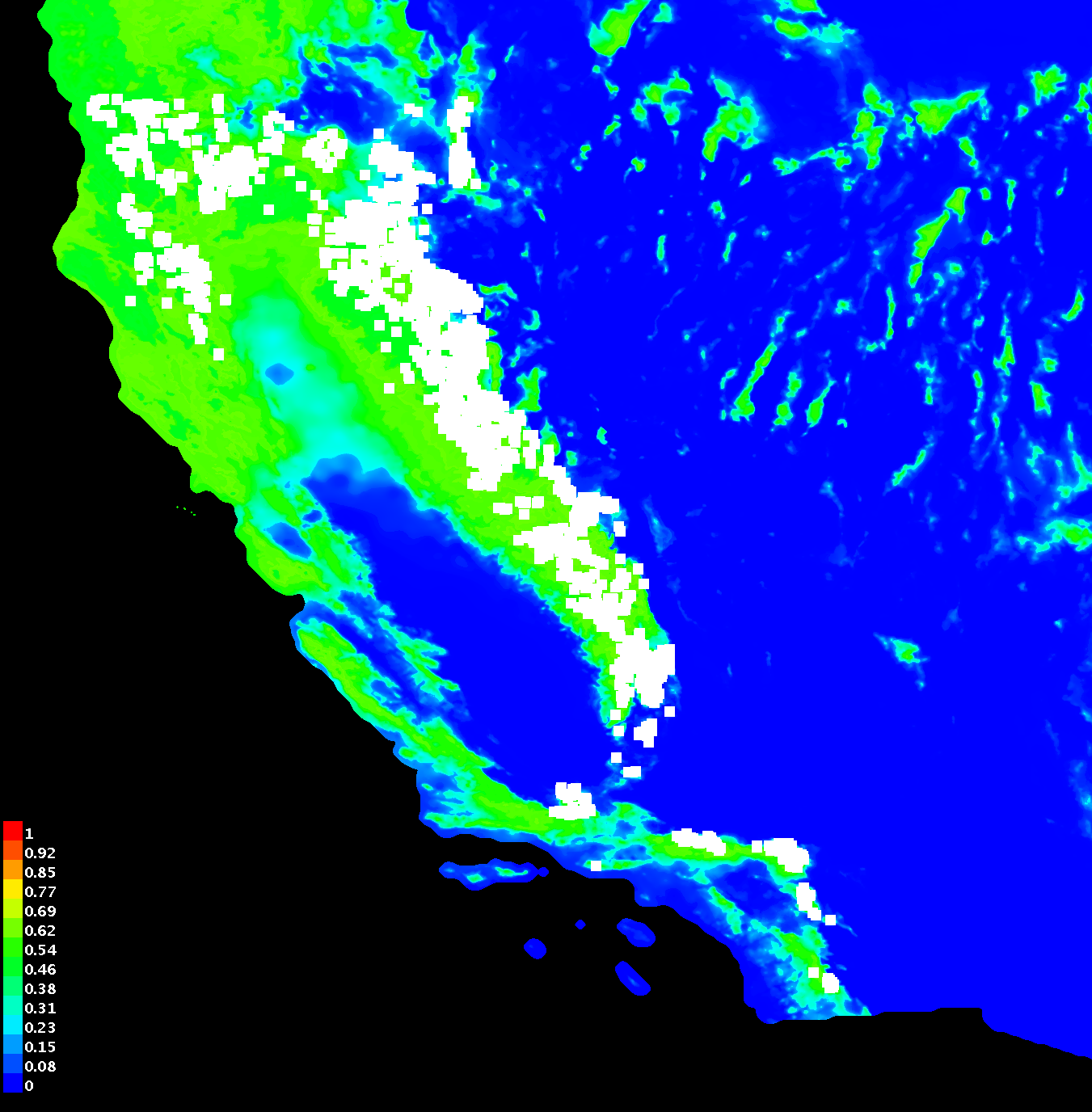
Each output folder will contain a .html webpage that summarizes the
model's information, including the predicted species distribution
overlayed on a map and several performance curves. Cooler colors
(blue/green) indicate areas where the model calculates a low
probability of species presence and warmer colors (red/yellow) indicate
areas where the model calculates a higher probability of species
presence. White squares indicate the locations specified in your
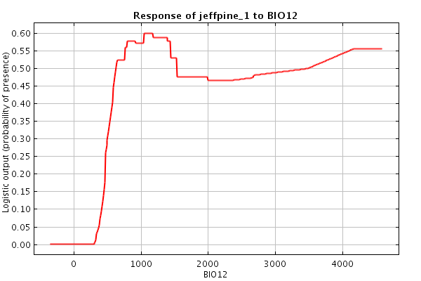
species presence file. For the response curve (middle figure),
the x-axis
represents a variety of climate values (in this case the annual
precipitation in mm) and the y-axis indicates the probability
of finding the species of interest in an area with any given annual
precipitation. So, the response curve below indicates that Jeffrey pine
trees
are most likely present in areas with an annual precipitation greater
than 600mm.
- Paste and label all four maps, response curves, and ROC curves in
your lab
write-up. For each response curve, construct a sentence or two
that describes the plotted relationship.
- Where is one area where each model over predicted the probability
of species presence? Why do you think this occurred?
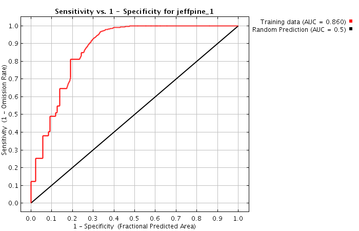
- What do the ROC curves tell you about each of these models?
Explain in a sentence or two.
- For each species, what is at least one other climate variable
that you
think you could add to improve the model’s performance? What would a
successful model look like?
Place your lab write-up (just one per group, please!) in hardcopy into
the submission box outside my office (Park 249) by Thursday, Sept. 23rd
at 2:30pm (class time) or submit it in-class then. Be sure to
keep
electronic copies of your lab write-up for next week's continuation of
this lab. Keeping your partners around would probably be best as
well. :-)
This lab is based on the Species
Distribution Modeling assignment developed by Park Williams, UCSB
Geography.